Simpson's paradox and the horrors of unobserved confounders

Posted on Jun 23, 2022

Let’s assume you have collected data from a hospital, where some patients are given a medicine and some are not. No experimental procedure was followed, you just collected whatever was out there and you want to check if taking the medicine causes improvements in health. With a bit of notational abuse, you want to check the effect of $T \rightarrow Y$. $T$ can be either 0 or 1 (whether someone was treated or not using the medicine), while $Y$ is a measurement of life quality – the higher the better. You plot the means and you see clear differences – see Figure 1.

Figure 1. Violin plot for treated and untreated groups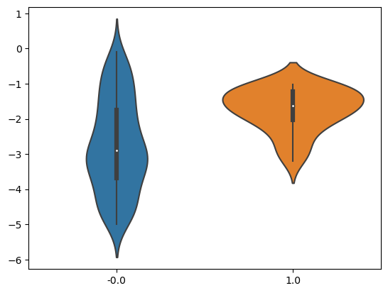

The difference in means is approximately $T_1 - T_0 \approx 1.0$ – this is termed the Average Treatment Effect ($ATE_X$). You run your t-tests, you get a p-value of $0.00012$ – good enough by most standards. At this point you are certain that you have gold in your hands, the medicine had a positive result. There are multiple ways you can calculate this effect; since we have no incoming features, we can just subtract the observed averages directly. Another (highly redundant) option would be to fit a regressor, loop over all our patients (i.e. data rows), force T to 1 or T to 0 and calculate averages.

Now, let’s assume that you somehow find a third feature $Z$ – let’s say that in some old scrap of paper someone was recording some other measurement for each patient. You now have two input features, the treatment and your new $Z$. You plug them in to a linear regression model and calculate the average, this time through the model (i.e. you force T=0 and T=1 for each patient and calculate the difference). To your surprise you get $ATE_X = -1$, exactly the opposite of what your initial calculations came up with. This is indeed a freaky event – knowing and taking into account another feature changed the results radically in the opposite direction – the medicine is now to be considered harmful!

Should you take this Z feature into account? Well, there is no way of knowing just by looking at the data, without any insights on how the data was generated. In our case, it was generated as follows:

def Z_confounder():
    return np.random.random(size=(observations, 1))

def T_treatment(Z):
    T = np.rint(Z + np.random.random(size=(observations, 1)))
    T[T > 1] = 1
    T[T < 0] = 0
    return T

def Y_outcome(Z, T):
    return -T + 5 * Z

z = Z_confounder()
t = T_treatment(z)
y = Y_outcome(z, t)

Just by reading the Y_outcome function, we can see that the $ATE_X$ is indeed -1. Y has both Z and T as inputs and T has Z as input. In this case, you should use Z as an input to your model. Judea Perl has a great piece of work here https://ftp.cs.ucla.edu/pub/stat_ser/r414.pdf discussing when you should and you shouldn’t use Z in detail (the whole phenomenon is called Simpson’s Paradox).

What if you have no clue what the data generating process is, or worse, you have no idea what other variables you need to measure? Well, you have no way of knowing whether your $ATE_X$ is biased, “no unobserved confounders” is one of the basic premises of this line of reasoning. You would need to do refutation work – how badly can you be damaged by unobserved features — and in our case it looks like this can be quite bit.

Most importantly, however, the whole premise of using observational data to measure effects allows for debates and interpretations that can go either way. As the saying goes “if you torture your data long enough, it will tell you whatever you want to hear”.

Hacky code for the above post